Symplectic Euler

A simple symplectic integrator

Overview

As you’ll recall one of limitations of Explicit Euler is that it does not conserve energy very well. Meaning that over finite timescales it can either introduce enough energy that the system becomes unstable, or bleed away all the energy until the system becomes static. This phenominon is known as Energy Drift. In this article we are going to learn about a class of numerical methods that don’t suffer as badly from this problem.

Vector Flows

Given an ordinary differential equation (ODE) like \begin{equation} \frac{\partial y}{\partial t}=g(t) \end{equation}

one can think of it as defining a vector field much like the force fields we discussed in Force Generators. If we denote by $y(t)$ a solution to the above ODE then the arrows of the vector field describe it’s rate of change. These arrows, taken together, are called the flow of the ODE. The flow is often written as a function $\phi_{t}$ that evolves a solution $y(t)$ forward. $\phi_{t+h}(y)$ = $y(t+h)$

Note: I very carefully used the phrase “a solution” above instead of “the solution”. That is because an ODE alone does not uniquely define a single solution $y(t)$ but a whole family of solutions. To select a unique solution out of this family you also need initial conditions. For example $\frac{\partial y}{\partial t}=y(t)$ has the family of solutions $y(t) = Ae^{t}$ for any constant A. If however I also knew that $y(0) = 1$ then I know that A must be 1 and hence I have the unique solution $y(t)=e^{t}$

The wikipedia article has this nice diagram to help visualize this

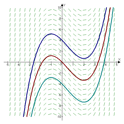
The curves are called integral curves and they represent solutions to the ODE that is described by the flow. You can think of each curve as representing a different set of intiial conditions for the system.

Hamiltonian Mechanics

Hamiltonian mecahnics is a deep topic that I won’t dive into here. Suffice to say that it’s a way of mathematically describing the universe that is exactly equivalent to Newton’s Laws. In fact Physicsts don’t really deal much with Newton’s Laws anymore, prefering instead to work with Hamiltonian Mechanics. However Newtonian mechanics is easier to understand intuitively so game engines tend to stick to this older way of doing things.

For our purposes when I say a system satisifies Hamilton’s Equations what I’m really saying is that the system behaves physically. Like Newton’s Second Law Hamilton’s Equations are a set of ODEs.

Important properties of Hamiltonian Systems

There are 2 important properties that all Hamiltonian systems have as far as this article is concerned.

Energy Conservation: Along a given integral curve energy is constant
Symplicity : Phase space area is conserved.

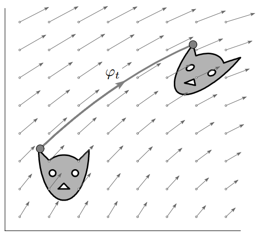
That last property seems to come out of nowhere. What even is phase space? Well phase space is an abstract way of describing all the possible states a system might take on. It is described by considering the positions and momenta of each entity in an $n$ component system as a seperate axis of $\mathbb{R}^{2n}$ . Here’s an example of what it would look like if you had a 1D system (a particle) whose allowed position and momentum values took on the shape of a cat in phase space. As the system evolves over time the allowed positions and momentums change, but the total area is conserved.

Why is symplicity important? I wish I had a intuitively satisfying answer but I don’t. It turns out that symplicity completely defines Hamiltonian systems. That is: any ODE whose flow $\phi_{t}$ is sympletic satifies Hamilton’s Equations and all ODEs that satisfy Hamilton’s Equations are symplectic. See theorem 2.6 in this book for a proof of this statement

If something is so important that it completely characterizes all possible physical systems its definetly worth conserving. But here’s where we run into a snag. Pretty much all the common methods for solving ODEs are based on power series expansion of the derivative. We’ll be talking more about this in the next article but this is exactly what we did for Explicit Euler. It turns out that it is impossible to have a numerical method formulated in this way that conserves both energy and area. (See Long-time energy conservation of numerical integrators by Ernst Hairer for a summary).

All is not lost however. Although we cannot have both, there is a famous result that gaurentees “nearly complete” energy conservation for symplectic methods. The exact statement of this theorem involves some terminology we haven’t spoken off, but suffice to say that for our purposes symplectic methods are the best we can hope for.

Symplectic Euler

So we have learned that Symplectic Integrators are the class of numerical methods that preserve area. What’s an example of such a method? The aptly named Symplectic Euler. \[ v_{f} = v_{i} + h\frac{F}{m} \] \[ x_{f} = x_{i} + hv_{f} \] Looks familar doesn’t it. Lets compare it to Explicit Euler. \[ v_{f} = v_{i} + h\frac{F}{m} \] \[ x_{f} = x_{i} + hv_{i} \] Can you spot the difference? It’s in the second equation. The update rule for position depends on the updated velocity, not on the intiial velocity. Amazing that such a small change can have such a huge impact.

All this comes back to the conversation we had about when to apply our approximations back when we developed Explicit Euler. If you’ll recall I said we could just as easily define the left hand side of our limit approximation as $v_{f}$ instead of $v_{i}$ . Turns out if you do that you get a way better integrator. Who knew! (I knew).

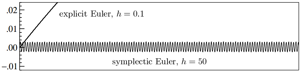
This image is a plot of Energy as a function of time and highlights the difference between Explicit Euler and Symplectic Euler. As you can see although Symplectic Euler does not exactly conserve energy from moment to moment, it does a much better job than Explicit Euler. In fact they had to turn the step size on Symplectic Euler way up to make the wiggles more noticable (recalling that a higher step size generally means a less physically accurate simulation).

Here’s the code for Symplectic Euler (.h,.cpp). It’s so similar to Explicit Euler there’s no point in talking about it in detail.

Results

After implementing Symplectic Euler our orbits are much more stable. However that doesn’t mean we are done with the topic of time integration. There are still other important properties of numerical solvers to discuss.